Fantasy Football Daily Fantasy

Print

Thoughts on “The Correlation Matrix that Answers Every Question You’ve Ever Had About DFS Stacking”

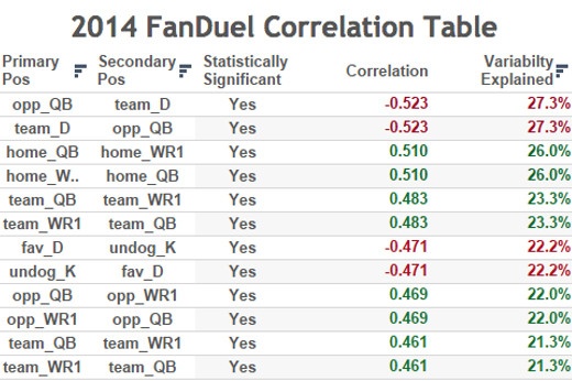
RotoViz is one of my go-to sources for quality, data-informed fantasy football research. But the take-aways from “ The Correlation Matrix that Answers Every Question You’ve Ever Had About DFS Stacking" are bit too black and white for me. The author might agree. “Truth be told, you might still have questions after reading this post. In fact, you might have more questions…”

Fact.

The Data

In most data driven research problems, roughly 90% of a data analyst’s time is spent on getting and cleaning the data. This has to be done prior to any analysis and frames any conclusions that can be made from the results.

In this article, there is no insight into the data used. Single week, year, multiple years? Scoring format? Number of samples?

No clue.

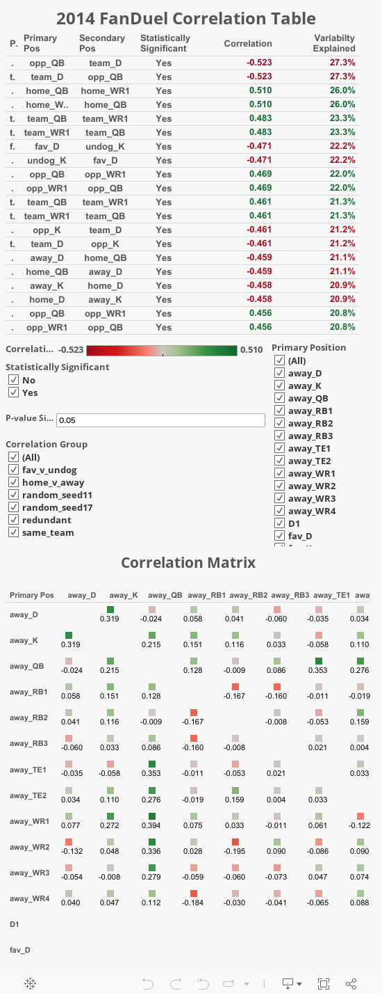
How was the data constructed with the opposing team players? How did the researcher determine which was team X and which was team Y? Home vs away? Favored vs underdog? Random? Did the researcher even think to avoid redundancy, stacking Team A’s K with Team B’s D and then Team B’s D with Team A’s K?

Because of the below x team correlation values being the same as those for team y, I highly suspect redundancy is an issue in any x,y correlations. For example, the WR2 QB1 correlation for the x teams look to be exactly the same as those in the y teams (as do every other pair compared in x and y).

x.WR2 x.QB1 0.39

y.WR2 y.QB1 0.39

I used player week data from 2014 based on FanDuel scoring as my source data (the week 12 match-up between KC and OAK was for some reason missing from the source file). In creating a data set to compare against the article’s results, I actually found it necessary to create multiple data sets to critique some of the take-aways of the author. First, to compare relationships within a team I created a data set with every team week including scores for K, D, QB1, QB2, RB1, RB2, RB3, RB4, WR1, WR2, WR3, WR4, WR5, WR6, TE1, and TE2. Roster depth was determined by weekly salary.

Avoiding the redundancy issue caused by taking this table and simply pairing each team with their opponent for that week is important. This causes a duplication of every data point reflected over the y=x line. This may cause an increased scatter in the data and/or inflated p values due to the increased sample size. Since there are multiple ways to consider match-ups, I created 4 match-up tables:

• Favorites vs. Underdogs (Based on spreads sourced from http://www.footballlocks.com) (255 cases)
• Home vs. Away (London games and the relocated Jets@Buffalo game were omitted) (251 cases)
• Random Selection 1 of Team A vs Opponent (255 cases)
• Random Selection 2 of Team A vs Opponent (255 cases)

For comparisons sake, I also created the redundant table.

Correlations

Correlations don’t tell the whole story. Just because something has high correlation doesn’t mean the linear relationship is especially influential. You need to consider the actual slope of the regression line to determine the impact one variable has on another in the comparison model. The question we really want to be able to answer is: "How many points are we expected to add to our team by utilizing a particular stack?”

P values are omitted. Many of the r values are likely statistically insignificant and yet they are all shared as meaningful in the article’s matrix and table. The claims made in takeaway number 6 are likely wrong. With such small correlation coefficients, I expect the p values to be high (unless the sample is extremely large) suggesting an insignificant linear relationship. So, to claim that x.QB1 has a negative correlation with y.WR1 and positive with y.WR2 would be wrong.

Without further tests, the claim in takeaway number 1 that the correlation between x.WR2 (and the not mentioned x.WR3) and x.QB is higher than that with x.WR1 is presumptive. The values are close enough that, depending on the sample, the difference may be insignificant. And as mentioned earlier, the slopes/influence would tell a more useful story.

The r values (correlation coefficients) themselves are hard to interpret. It would have been wise to provide r^2 values, as well. This would then express the percentage of variation explained in one variable by the other. For example, the strongest linear relationship in their study, K vs opposing D, had a -0.50 correlation. A kickers performance could explain 25% of an opposing D’s performance.

Further, correlations only check for linear relationships, which I do expect in this data as well, but any quadratic or logarithmic relationships may be overlooked.

In “tCMtAEQYEHADS”, the author claims kicker versus opposing defense has a -0.5 correlation statistic. Summary of the related correlations from my data:

• favorite K vs underdog D -0.38
• undog K vs favorite D -0.47
• home K vs away D -0.41
• away K vs home D -0.46
• rand(1) team K vs opponent D -0.42
• rand(1) opponent K vs team D -0.36
• rand(2) team K vs opponent D -0.39
• rand(2) opponent K vs team D -0.46
• redundant team K vs opponent D -0.44
• redundant opponent K vs team D -0.44

So, you can see the importance of framing your data for the reader.

In take-away 2, the author states a RB1 has a negative correlation with all TEs and WRs from the same team. In my study, only RB1 and WR1 (using the Random 1 set) had a statistically significant linear relationship (although the correlation was still small at 0.11) and it was positive, not negative.

Take-aways 3 and 5 are supported in my data. Take-away 4 of opposing Ks and Ds having a negative correlation is also supported, but the same can be said for a D and any opposing offensive player, especially QB (even more so than K).

Take-away 6 is partially supported. A WR2 does seem to have a statistically significant positive correlation with the opposing QB (again, using the Random 1 set). However, the linear relationship between the WR1 and the opposing QB is statistically insignificant.

Finally in take-away 7, based on my data (again, using the Random 1 set), opposing QBs, RB2s, WR1s, WR2s and TE1s do not have significant linear relationships. Opposing RB1s and WR4s do have a negative linear relationship, although not a high correlation. Opposing WR3s do have a positive linear relationship, although, again not a high correlation.

We could easily have different (and more useful) take-aways when considering favorite vs. underdog or home vs. away match-ups. That just reiterates the importance of framing the questions you’re trying to answer as a researcher.

Next Steps

• Expand data set beyond 2014.
• Review scatter plots for non-linear relationships
• Run Principal Component Analysis on tables to determine grouped relationships instead of paired relationships.
• Create regression models to determine the strength of the influence of explanatory variables on response variables.

Chasing Upside in Stacking Teammates

Below are the results of an ongoing stacking study (limited to players from the same team) with a slightly different approach. I believe this is more actionable information. The question that I’m intending to answer is, “if I can identify a top performing player at position X should I stack them with a teammate at position Y?”

1. Using 2014 FanDuel data, identify top N players each week at primary position.
2. Stack with secondary position limiting to a certain depth on roster (WR1, WR2, etc.)
3. Compare stacked player to alternative at similar salary (within 100 dollars)

• Top 5 Qb with WR1 +6.5 points better than alternative at similar price (313 cases)
• Top 15 WR with QB1 +3.9 points better than alternative at similar price (392 cases)
• Top 5 Qb with WR2 +4.0 points better than alternative at similar price (579 cases)
• Top 5 Qb with WR3 +1.1 points better than alternative at similar price (691 cases)

• Top 5 Qb with TE1 +1.3 points better than alternative at similar price (385 cases)
• Top 5 TE with QB1 +2.9 points better than alternative at similar price (126 cases)

• Top 5 QB with RB1 +2.2 points better than alternative at similar price (234 cases)
• Top 10 RB with QB1 +1.2 points better than alternative at similar price (260 cases)
• Top 5 QB with RB2 statistically insignificant relationship (538 cases)

• Top 5 QB with D -.9 points worse than alternative at similar price (512 cases)
• Top 5 D with QB1 statistically insignificant relationship (139 cases)

• Top 5 QB with K +.9 points better than alternative at similar price (684 cases)
• Top 5 K with QB1 +2.2 points better than alternative at similar price (127 cases)

• Top 10 RB with WR1 statistically insignificant relationship (620 cases)
• Top 15 WR with RB1 +0.8 points better than alternative at similar price (672 cases)

• Top 10 RB with TE1 statistically insignificant relationship (920 cases)
• Top 5 TE with RB1 +1.6 points better than alternative at similar price (290 cases)

• Top 10 RB with D +0.6 points better than alternative at similar price (1034 cases)
• Top 5 D with RB1 statistically insignificant relationship (196 cases)

• Top 10 RB with K +0.9 points better than alternative at similar price (1211 cases)
• Top 5 K with RB1 +1.9 points better than alternative at similar price (264 cases)

• Top 15 WR with TE1 statistically insignificant relationship (1258 cases)
• Top 5 TE with WR1 statistically insignificant relationship (324 cases)

• Top 15 WR with D statistically insignificant relationship (1556 cases)
• Top 5 D with WR1 statistically insignificant relationship (293 cases)

• Top 15 WR with K +0.8 points better than alternative at similar price (2028 cases)
• Top 5 K with WR1 +1.6 points better than alternative at similar price (285 cases)

• Top 5 TE with D statistically insignificant relationship (493 cases)
• Top 5 D with TE1 statistically insignificant relationship (383 cases)

• Top 5 TE with K +0.9 points better than alternative at similar price (632 cases)
• Top 5 K with TE1 statistically insignificant relationship (388 cases)

• Top 5 D with K +3.0 points better than alternative at similar price (600 cases)
• Top 5 K with D +2.9 points better than alternative at similar price (471 cases)

Take-aways:

• Stacking top QBs with their offensive team-mates is highly suggested
• Beside top QB/WR stacks, top K/D stacks offer the most expected benefit.
• Most of the intra-team top stacks have a positive expected return over the alternative, a handful of stacks do not have significant advantages over an alternative, but pairing a top 5 QB with their Defense is the only negative stack on a team.

Using any of these positive correlations should be safe advice in any cash games. More research needs to be done into potential upside/limits and application in GPPs. Hopefully, you can leave this better informed about making stacking decisions in your FanDuel lineups. Hope to see you in the FanDuel Lobby looking for your next mark... and I hope I'm not it.

Finally, I’d be remissed if I critiqued the RotoViz Correlation Matrix without providing some alternative.

Jared Smola, Lead Analyst

Jared has been with Draft Sharks since 2007. He’s now Lead Analyst, heading up the preseason and weekly projections that fuel your Draft War Room and My Team tools. He currently ranks 1st among 133 analysts in draft rankings accuracy.